Status: v2.0 draft, October 20, 2026. Working hypothesis. Survives, with conditions. It writes down an explicit non-local guidance law that can’t send signals, and says openly that it needs a cosmic time slicing (section 3).
Authors: Christopher B. Hanni (Chief Architect), with Gem (Guardian Navigator). Referee pass and edits by Claude.
References (all links checked):
- J. Maldacena and L. Susskind, “Cool horizons for entangled black holes” (ER = EPR), Fortschr. Phys. 61, 781 (2013): https://arxiv.org/abs/1306.0533
- S. Ryu and T. Takayanagi, “Holographic derivation of entanglement entropy from AdS/CFT”, Phys. Rev. Lett. 96, 181602 (2006): https://arxiv.org/abs/hep-th/0603001
- M. Van Raamsdonk, “Building up spacetime with quantum entanglement”, Gen. Relativ. Gravit. 42, 2323 (2010): https://arxiv.org/abs/1005.3035
- D. Dürr, S. Goldstein and N. Zanghì, “Quantum equilibrium and the origin of absolute uncertainty”, J. Stat. Phys. 67, 843 (1992): https://arxiv.org/abs/quant-ph/0308039
- D. Dürr, S. Goldstein, T. Norsen, W. Struyve and N. Zanghì, “Can Bohmian mechanics be made relativistic?”, Proc. R. Soc. A 470, 20130699 (2014): https://arxiv.org/abs/1307.1714
- A. Valentini, “Signal-locality, uncertainty, and the subquantum H-theorem. I”, Phys. Lett. A 156, 5 (1991): https://doi.org/10.1016/0375-9601(91)90116-P
1. The premise of the test
Part 6 showed that one particle’s interference pattern comes from a 3D superfluid wake in the Plenum. It also flagged the hard limit: a local 3D wave moving at can’t produce the correlations of entangled particles (Bell–CHSH). For entangled particles the phase lives in -dimensional configuration space. A measurement on particle A changes the guidance of a distant particle B at once.
Part 6 set the bar for this part:
- The thread. How do two distant knots stay connected without a large wormhole that would collapse?
- The law. What equation carries the non-local link, and why can’t it be used to send faster-than-light messages?
- The frame. Does the law need a preferred time slicing, and how does that fit with Lorentz symmetry?
2. ER = EPR, mainstream and Plenum
2a. The mainstream idea
In GR, an Einstein–Rosen (ER) bridge is a wormhole that can’t be crossed. In quantum mechanics, Einstein–Podolsky–Rosen (EPR) entanglement is a joint state that doesn’t split into two separate ones, and it violates Bell’s inequality (). Building on the Ryu–Takayanagi formula, , and Van Raamsdonk’s argument that entanglement builds spacetime, Maldacena and Susskind proposed ER = EPR: entangled particles are linked by tiny wormholes. For a single pair of spins, though, a smooth classical wormhole would have to be Planck-sized, where classical GR breaks down.
2b. The Plenum version: one braid, two ends
In the True Atom, 3D space (the Now Set ) isn’t the fundamental container. It’s a projection from the unmanifest Null Set (). When one parent knot (or a down-conversion crystal) splits into an entangled pair that fly apart, they don’t cut their shared fibers. Gem describes the link with the Gauss linking integral:
In 3D the two cores may be far apart. Along the fiber beneath space, the connecting tendril has zero length: two ends of one braid.
Referee note (Claude):
- ⚠️ The linking number is a whole number. For two closed curves the Gauss integral is always an integer, so it can’t take the fractional values () used elsewhere for “lower overlaps”. Entanglement, by contrast, comes in degrees (from none to maximal). So “entanglement = linking” is a postulate that still needs a continuous measure. It might be a linking density, or the overlap of the two knots’ phase fields.
- Credit and difference. Maldacena–Susskind’s ER = EPR lives in holography (AdS/CFT), where the wormholes are quantum objects. The Plenum’s tendril is a different proposal that borrows the name. The page should keep the two apart.
3. The Part 6 bar: frame, law, no signaling
3a. Yes, it needs a time slicing: the cosmic Plenum frame
Bell, and later Dürr, Goldstein, Norsen, Struyve and Zanghì (2014), showed that a pilot-wave theory reproducing entanglement for distant measurements needs a foliation: spacetime sliced into “nows” , along which the link acts.
In empty space, picking such slices feels arbitrary. The Plenum already has natural ones: the slices of constant cosmic time, at rest with the relaxing medium. That’s the frame where the CMB looks the same in all directions. Gem defines it with the same relaxation field as Part 4:
So the theory has a preferred slicing underneath, while every local laboratory result stays Lorentz invariant.
Referee note (Claude): ✅ Stated openly, which is what the bar asked. It’s also consistent with Part 4: the same frame shows up there, and at first post-Newtonian order it’s invisible in gravity tests too (Part 4, section 8). Dürr et al. note that the slicing can even be built from the wavefunction or a field like ; that’s the covariant way to say it.
3b. The explicit guidance law
For spin-½ knots at positions on the slice , with joint state and density , knot moves with:
and feels the joint quantum potential:
- Not entangled: , so splits into , and each knot’s motion depends only on itself. No link.
- Entangled: doesn’t split. When Alice runs knot 1 through a Stern–Gerlach magnet, its wave splits into up and down channels, and that instantly changes the guidance of Bob’s knot 2. The result is the quantum correlation and .
Referee note (Claude):
- ✅ This is the standard de Broglie–Bohm–Pauli law, so it reproduces quantum mechanics exactly. That’s a pass, and it means the tendril picture makes no new prediction here. Nothing in the equations uses ; the physics is all in .
- Small factor fixed. With , the spin term is . Gem’s draft had an extra ½. This is the Pauli (slow-particle) form; the Dirac version uses the current .
3c. Why Alice can’t signal Bob
Bob’s knot responds to Alice’s setting at once, yet she can’t use it to send a message. The reason is quantum equilibrium (Dürr, Goldstein & Zanghì 1992; Valentini 1991):
- The continuity equation guarantees that an ensemble starting with positions distributed as stays that way.
- Alice’s and Bob’s local operations commute, so the evolution factorizes, .
- Bob, who doesn’t know where Alice’s knot is, sees only his marginal distribution:
Because , Alice’s setting drops out. The preferred slicing is also invisible in equilibrium. Signaling, or detecting the slicing, would require a non-equilibrium state, (Valentini).
Referee note (Claude): ✅ Correct and standard. Gem suggests CATBT’s picosecond window (Part 7) as a place where non-equilibrium might briefly appear. That’s speculative, and any such effect would also be a Lorentz-violation signal, so existing precision tests already bound it. Worth stating as a long shot, not an expectation.
4. The original Weyl “Bridge Equation”, updated
The May draft used the conformal bridge . As Part 2 showed, a purely conformal metric bends light by zero. In v2.0 the bridge between entanglement and geometry has two parts:
- Space slices. In the static limit the slice metric is conformal, . Gem proposes that tracks the local entanglement deficit, in the spirit of Ryu–Takayanagi: .
- Spacetime. Time and space factors have opposite signs in the exponent (, ). That’s what gives GR’s light bending, .
Referee note (Claude): 🟡 The second point is solid (Part 2). The first, as entanglement deficit, is a hypothesis with no equation yet linking a given entangled state to a given . Label it as the next thing to derive.
4a. Newton’s constant from thread density
If the Shell Zone carries one entanglement thread per area , matching the area law gives:
Referee note (Claude): 🟡 Dimensionally consistent. It says , so the knot size is near the Planck length. A useful cross-check: then – GeV, which passes every dispersion bound in Part 7 by a wide margin (they need only GeV). The tension: CATBT’s relaxation time is picoseconds, about 31 orders of magnitude slower than . One of the two needs explaining (Part 7, section 5).
5. Checks: what passes, what’s open
| Check | Status | Plenum mechanism | Still needed |
|---|---|---|---|
| Bell–CHSH violation () | ✅ passes | de Broglie–Bohm–Pauli guidance on the cosmic slicing | — (identical to quantum mechanics) |
| No signaling | ✅ passes | Quantum equilibrium; Alice’s setting cancels in Bob’s statistics | Bound possible non-equilibrium |
| Preferred slicing vs. Lorentz symmetry | ✅ stated openly | Cosmic Plenum (CMB) frame, ; hidden in equilibrium | — |
| Entanglement = linking | 🟡 pure states derived from the guidance law (section 8) | Missing local spin: ; general case = Wootters in each knot’s spin-flipped frame | Mixed states from the guidance law |
| from entanglement | 🟡 hypothesis | Ryu–Takayanagi-style area law | An equation from state to |
| from thread density | 🟡 scaling | near the Planck length | Packing constant; picosecond explained as shower clearing (Part 7, section 6) |
6. Fourth pass (Oct 20, night): a continuous measure of linking
Linking numbers of closed loops are whole numbers, but entanglement varies smoothly (the concurrence runs from 0 to 1). Gem’s answer uses two established results:
- Open strands wind by any amount. The tendrils between knots and aren’t closed loops; they end on the knots. For open strands, the winding of one around the other is a real number, not an integer (Berger & Field 1984, J. Fluid Mech. 147, 133).
- Bundles average it. Each knot is tied to the Plenum by a bundle of fibers. Averaging the pairwise linking over two bundles gives a smooth number, Arnold’s asymptotic linking (Arnold 1974; Moffatt 1969, J. Fluid Mech. 35, 117).
Gem then proposes that for the braided fraction of the bundles is
which equals the concurrence of that state.
Referee note (Claude):
- ✅ The integer problem is solved. Both references are real and say what Gem says: open-strand winding and bundle-averaged linking are continuous.
- 🟡 The formula is matched, not yet derived. Setting the braided fraction to is chosen to equal the concurrence. A derivation would start from the knots’ guidance law (section 3) and show that state produces that braid.
- ⚠️ Key requirement: local operations can’t change it. Entanglement can’t be changed by acting on one particle alone. But the winding of open strands does change if you twist one end. The measure has to be defined so that twisting knot by itself leaves it unchanged (for example, by measuring winding relative to each knot’s own frame).
- ⚠️ Mixed states need Wootters’ general formula, not ; the measure should reproduce that too.
7. Fifth pass (Oct 20, late night): a measure local twists can’t change
Gem’s fix: measure each knot’s braiding against its own spin-flipped frame instead of a lab axis. The spin flip uses , and every single-knot rotation obeys , so a twist of one end cancels out. For any two-knot state, pure or mixed, this is Wootters’ construction (1998, quant-ph/9709029):
Here the are the square roots of the eigenvalues of , largest first. Local twists change only by a similarity transform, so the and don’t change. For the pure state of section 6 it gives .
Referee note (Claude):
- ✅ Both requirements are met: invariance under local twists, and mixed states. I checked the identity and the pure-state limit.
- 🟡 Honest reading, as Gem says: this adopts the standard quantum measure and gives it a geometric meaning (braiding read in each knot’s own spin frame). That’s a structural correspondence, not yet a derivation. The next step would be a braid observable of the Plenum, computed from the guidance law, that comes out equal to .
8. Sixth pass (Oct 20, late night): a braid observable from the guidance law
Gem proposes the Bohmian cross-helicity: integrate knot ’s guidance velocity against the curl that ’s velocity has with respect to ’s position,
For a product state doesn’t depend on , so . Gem proposes that for the entangled state of section 6 its normalized size is .
Referee note (Claude):
- ✅ Zero for product states: correct.
- 🔧 But it is also zero for this entangled state. Take the spin state with each knot in its own wave packet, . In the Bohm–Pauli guidance law, , where is constant. Nothing in depends on , so the cross-curl vanishes for every . Spin entanglement only reaches the trajectories once a measurement (a Stern–Gerlach magnet) ties spin to position.
- ✅ What the guidance law does show: look at the size of the spin term. Each knot’s local spin vector shrinks as entanglement grows: . For any pure two-knot state, the exact identity
holds (). Read in the Plenum picture: the part of a knot’s spin twist that can’t be seen locally is the part braided with its partner. It is derived, not matched; it doesn’t change under local twists (only the vector’s length enters); and it uses the guidance law’s own spin term. - ⚠️ Limit: this works for pure states. For mixed states, a short local spin vector can also mean ordinary classical uncertainty, so the general measure stays Wootters’ (section 7).
9. Seventh pass (Oct 20, evening): adopted, plus where the bridge honestly stands
Gem adopts the local-spin measure, . The Plenum reading: a knot’s total twist has length 1; entanglement moves part of it into the shared tendril, where it can’t be seen locally. Gem extends this to mixed states: local decoherence is twist leaking into the substrate.
Referee note (Claude):
- ✅ The decoherence reading is consistent with standard physics. Any mixed state can be written as part of a larger pure state (purification), so “twist braided with the environment” is a fair picture of decoherence.
- ⚠️ But one knot alone can’t tell the two cases apart. A short local spin vector can mean braided twist or plain ignorance. Only the joint system shows the difference.
Have we reconciled quantum mechanics and relativity?
Chris asked this directly, so here is the honest status.
- What is done: a single framework where classical gravity matches GR in every tested regime at first post-Newtonian order (section 12 of Part 4). It differs at 2PN, which can be tested. In the same framework, quantum mechanics runs as a pilot wave on the Plenum’s time slicing: Bell violation, no signaling, and now a geometric reading of entanglement. They coexist consistently. This is a real and respectable position, close to the “hypersurface Bohm–Dirac” line of work by Dürr, Goldstein and colleagues.
- What isn’t done yet: gravity here is still classical, sourced by quantum matter. A full reconciliation has to say what happens when the source is in a superposition. Is the Plenum’s quantum, or classical but slightly noisy? The second option is serious physics: Oppenheim’s classical-gravity theory (2023) requires a trade-off between gravitational noise and decoherence that experiments can check. Black-hole information and the behavior at the Planck scale are also open.
- The sharpest test coming: tabletop experiments to see whether gravity alone can entangle two masses (Bose et al. 2017; Marletto & Vedral 2017). If gravity entangles, must carry quantum information, and a purely classical is ruled out. If it doesn’t, classical-gravity frameworks like this one gain ground. The Plenum should state its prediction before the result arrives.
10. Eighth pass (Oct 20, evening): the prediction is on the board
The True Atom’s prediction for the gravity-entanglement (BMV) experiments: no gravity-mediated entanglement, together with mass-dependent decoherence driven by the substrate. The reasoning: is a collective, hydrodynamic variable of the substrate, not a quantized spin-2 field. Putting a mass into a spatial superposition splits its Render Wake, and the substrate’s restoring tension collapses it, much like Penrose’s gravitational collapse or Oppenheim’s noisy classical gravity.
Referee note (Claude): a falsifiable prediction stated in advance. That’s exactly right. Three things make it sharper.
- ⚠️ Say how quantum matter sources . This one rule decides the prediction.
Also note that the textbook two-body term inside the Schrödinger equation is what predicts entanglement. The Plenum is saying that term is not fundamental, which is a big claim and worth stating openly.
- sourced by the average mass density (the Schrödinger–Newton picture): no entanglement, but the equation becomes nonlinear. Page & Geilker’s 1981 experiment already argues against this.
- sourced by the actual Bohmian particle positions: natural for a pilot-wave theory (Struyve has explored it), but it must not allow signaling.
- classical but noisy (Oppenheim 2023): then the noise level must respect torsion-balance bounds.
- ✅ A number for the decoherence (machine estimate). Use the Diósi–Penrose rate for a uniform diamond sphere, with .
- For BMV-style masses kg (m) with superpositions split by m: J, so ms.
- The gravitational phase builds at about rad/s at m.
- So the superposition would collapse roughly 300 times faster than entanglement could form. The collapse itself would be the signal.
- At kg, s.
- ⚠️ Watch the existing limits. The parameter-free Diósi–Penrose model is already strongly constrained by the Gran Sasso underground radiation search (Donadi et al., Nature Physics 2021). Any Plenum collapse rate has to sit inside those limits, so it needs a stated smearing length or noise level.
Honest framing: this is classical gravity plus quantum matter with a sharp, testable prediction. It is not yet quantum gravity. If BMV-type experiments do see gravitational entanglement, this version of the Plenum is falsified, and that’s what makes it science.
11. Ninth pass: Consistent Coexistence, and Bohmian sourcing
Banner adopted: Consistent Coexistence. Gem chooses the sourcing rule: is sourced by the actual Bohmian positions, . The big claim is stated openly: the textbook term in the quantum Hamiltonian is an effective description, not fundamental. To pass the Gran Sasso bounds, the substrate’s noise is colored: it has a high-frequency cutoff and a smearing length m.
Referee note (Claude):
- ⚠️ The no-signaling proof in section 6 needs redoing. That proof assumes the wave function evolves on its own, independent of the actual positions. With Bohmian sourcing, (set by the actual positions) feeds back into the wave equation. Then is no longer automatically preserved (equivariance), and quantum equilibrium, the thing that blocks signaling, has to be shown again. Struyve treats this kind of coupling as an approximation for exactly this reason. This is the key open item for this choice.
- ✅ A bonus prediction falls out. In the BMV setup, mass 2 feels gravity only from the branch where mass 1 actually is. So its two branches pick up a relative phase whose sign depends on the hidden position of mass 1, 50/50 from run to run. Averaged over runs, that looks like dephasing with no entanglement: fringe visibility , and the entanglement witness stays below threshold. This comes directly from the sourcing rule, before any collapse mechanism is added.
- 🟡 The smearing length passes the current bound. Donadi et al. (2021) need Å, and m is far above that. Because is smaller than the 0.88 μm grain, the roughly 12 ms collapse estimate still holds. But and are currently chosen to pass the bounds. To count as a prediction, they must come from and fixed elsewhere (for example, Part 5’s core scale). Colored-noise collapse models are an existing literature to cite and compare against. “Suppresses X-ray emission entirely” should read “suppresses it below the current bounds”, with a number.
Where it stands: a classical-gravity, pilot-wave framework with two falsifiable signatures for BMV-type experiments: no entanglement, and dephasing/collapse at stated rates. The open items are written down. That’s a strong, honest place to stand.
12. Tenth pass: equivariance, the visibility signature, and colored noise
References (checked):
- W. Struyve, Semi-classical approximations based on Bohmian mechanics (arXiv:1507.04771, 2015).
- W. Struyve, Towards a novel approach to semi-classical gravity (arXiv:1902.02188, 2019).
- Background: W. Struyve, Pilot-wave theory and quantum fields, Rep. Prog. Phys. 73, 106001 (2010) (doi).
- S. L. Adler & A. Bassi, Collapse models with non-white noises (arXiv:0708.3624, 2007).
- S. Donadi et al., Underground test of gravity-related wave function collapse, Nature Physics 17, 74 (2021) (doi, arXiv:2111.13490).
1. Equivariance (Gem’s statement). On a single run, is just a time-dependent potential, so probability-current conservation holds along that run. Across an ensemble, though, each run evolves under its own Hamiltonian, so is preserved (equivariance) only approximately. The approximation fails once the gravitational energy differences between branches reach . Proving an exact version is an open problem.
Referee note (Claude): ✅ stated correctly. Note one thing honestly: BMV experiments are designed to reach , which is exactly where this approximation is weakest. So the no-signaling question and the BMV prediction live in the same regime. That’s worth a line in the paper.
2. The visibility signature. Averaging mass 2’s coherence over the 50/50 hidden branch of mass 1 gives :
There is no entanglement, and the visibility comes back periodically (revivals) as long as no collapse acts. ✅ This is the sharpest signature: a standard quantum-gravity entanglement analysis predicts the witness crossing threshold, while this predicts revivals with the witness staying below it.
3. Colored noise vs. Gran Sasso. With a Lorentzian cutoff and X-ray frequencies (10 keV), the emission is suppressed by .
Referee note (Claude):
- ✅ The arithmetic checks, and “below current bounds by a number” is the right wording.
- Even easier than stated. The Diósi–Penrose radiation rate scales as , and Donadi’s bound is Å. So even white noise with m sits about below the bound. Colored noise adds more margin on top.
- ⚠️ The low-frequency side still needs checking. A high-frequency cutoff does nothing for slow tests. Mechanical and heating experiments (cantilevers, LISA Pathfinder) have constrained collapse models at low frequency, so the Plenum’s noise has to be checked there too.
- ⚠️ from : put in the numbers. For example, if is Planck-sized and is centimetres, this gives about m, not m. Whichever scales are meant, they need to be stated so the result can be checked.
13. Eleventh pass: the low-frequency bounds
References (checked):
- B. Helou et al., LISA Pathfinder appreciably constrains collapse models (arXiv:1606.03637): measured noise fm s⁻²/√Hz; DP bound fm.
- M. Carlesso et al., Experimental bounds on collapse models from gravitational wave detectors (arXiv:1606.04581).
- A. Vinante et al., Narrowing the parameter space of collapse models with ultracold layered force sensors, PRL 125, 100404 (2020) (doi).
Gem’s numbers. At m, Gem uses . That gives about m s⁻²/√Hz for LISA Pathfinder (vs. the measured 5.2 fm s⁻²/√Hz), and roughly ten orders of magnitude below the cantilever noise. is now stated honestly as a phenomenological scale in m, with no first-principles derivation yet.
Referee note (Claude): ✅ The conclusion holds, with a wide margin. Two notes on the numbers:
- The formula may overstate the noise. For a uniform sphere with , the large- tail of converges even without the smearing. So the force noise tends to , independent of , with no boost. That gives about m s⁻²/√Hz for LISA Pathfinder, even further below. Please check the cited equation. Either way, the margin is –.
- Cantilever arithmetic. Gem’s own formula gives N²/Hz, not . Both are far below .
- Why LISA Pathfinder’s DP bound is so small (40 fm). It comes from the regime where the smearing resolves individual nuclei. At 100 nm, the solid looks smooth and that enhancement disappears, so 100 nm is safe.
Status: with Gran Sasso (section 12) and now the low-frequency tests, m passes every bound checked, at both high and low frequency. What remains is deriving it.
Follow-up (Gem + Claude, Oct 21): Gem confirmed the -independence using the exact uniform-sphere form factor .
- One correction (checked numerically). , not . So .
- The numbers that follow. Carried through Gem’s chain, this gives :
The earlier was the old formula.
- LISA Pathfinder: m s⁻²/√Hz.
- Cantilever: N²/Hz.
- Bottom line. The overall prefactor depends on the DP normalization convention. The margins ( below LISA Pathfinder, below the cantilever) don’t. ✅ Closed.
Next: Part 9, the Noosphere, global consciousness and the Omega field.
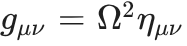 ):
 , the perfectly flat, frictionless substrate.
 , which warps the flat substrate into the curved spacetime metric we experience,
 . Gravity is simply the mapping of quantum information onto the fluid substrate.